Inspired by Valerio Velardo’s great resources on the applications of Deep Learning (DL) to audio I decided to train a convolutional neural network on Google’s Speech Command dataset. It contains one-second .wav audio files, each containing a single spoken English word. The simplicity of this data makes it a great starting point for a simple DL model.

The model has been trained on the following words: right, eight, cat, tree, bed, happy, go, dog, no, wow, nine, left, stop, three, sheila, one, bird, zero, seven, up, marvin, two, house, down, six, yes, on, five, off, four.

The main purpose of this project is approaching the use of deep learning for audio applications. To this end, it is quite a simple model, and therefore it will only process the first second of any audio file that is submitted to it. Audio sequences shorter than one second are padded with zeros at the end.

To test this model, upload an audio file with an utterance of one of the keywords listed above and submit the form.

Pick a file below or record it. Inferred word will appear here.

Make a recording here

Only the first second will be processed, speak as soon as you press the record button.

Record Stop

Overall architecture

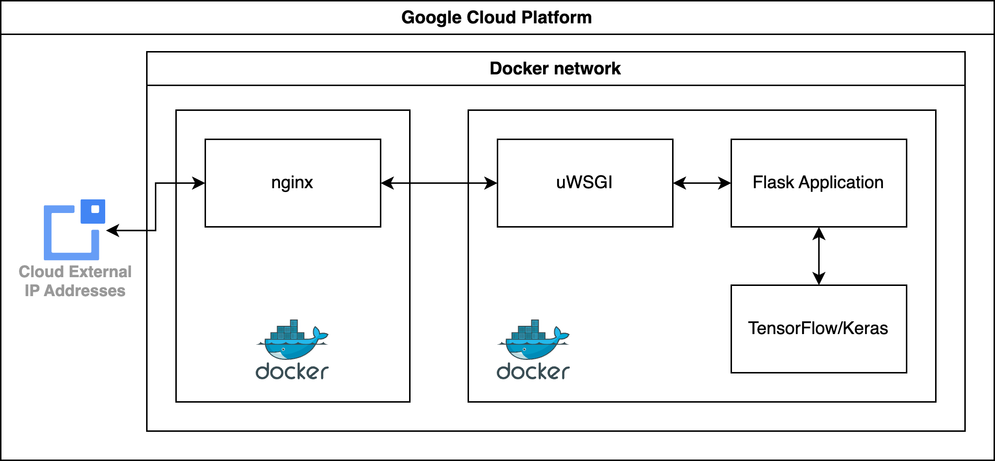
• The model is running on Tensor Flow and was built using Keras APIs.
• A Python Flask application is in charge to handle requests: it invokes the model, preprocesses the audio file and sends back the model’s output.
• Requests are made via HTTP POST calls to an nginx server that passes requests to the Flask application via uWSGI.
• nginx and Flask run on two separate Docker containers, both living in a Docker network.
• this sample application is deployed on Google Cloud Platform (GCP).

Audio preprocessing

Dataset

The dataset has 65000 one-second long utterances of 30 short words. The recordings originate from uncontrolled settings. This was intentional and by design, in order to collect samples that resemble real-world data. The recordings were then converted to a 16-bit little-endian PCM-encoded WAVE file at a 16000 Hz sample rate. The audio was then trimmed to a one-second length to align most utterances, using the extract_loudest_section tool. The audio files were then arranged into directories with each directory name labelling the word that is spoken.

Data split

I reserve 10% of the data for testing, meaning that this data will not be used to evaluate the model during training. The remaining 90% is split further, by using 10% for validation during training, while the rest is used to train the model.

Features

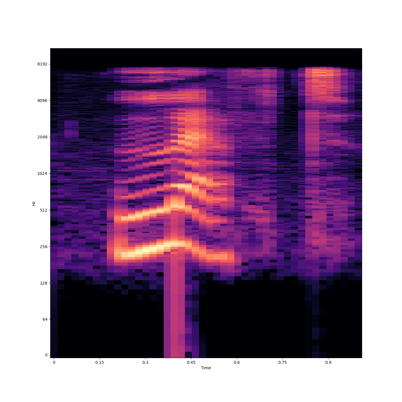
From each audio file I compute the Mel-Frequency Cepstral Coefficients (MFCCs). To compute MFCCs, one can first compute the Mel-Spectrogram.

A Mel-spectrogram is a time-frequency representation of an audio signal, where the frequency axis is transformed to the Mel scale. The Mel scale approximates human auditory perception and emphasizes the range of frequencies that are more important for speech recognition. To compute a Mel-spectrogram, you first obtain a short-time Fourier transform (STFT) spectrogram and then apply the Mel filterbank (a set of triangular filters) to the power spectrum. The result is a 2D representation that shows how the power in different Mel-frequency bands evolves over time.

Once we have the Mel-spectrogram, the log of the Mel-scaled power spectrum is computed, and a discrete cosine transform (DCT) is applied to the log-scaled Mel-spectrogram. The MFCCs are the coefficients resulting from the DCT. Typically, only the first few coefficients (e.g., the first 12-20) are used, as they contain most of the information relevant to speech recognition and audio classification tasks.

This post provides a comprehensive overview of MFCCs and filterbanks in the domain of speech processing.

For this model I use 13 coefficients. Since the MFCCs are also a 2D representation of the signal, they can be seen as images or snapshots of the audio file. In fact, they are indeed treated as images by the CNN.

Noise

The dataset also provides some noise that can optionally be added to the audio recordings in order to enrich the dataset. In this context I decided not to add any background noise.

Convolutional Neural Network

The network is made of three convolutional layers, and two dense layers. To deal with overfitting, at each convolutional layer an \(L2\) regularizer is applied, this adds a penalty term to the loss function, which encourages smaller weights. After a Rectifier Linear Unit (ReLU) activation, the output is normalized and downsampled with max-pooling. Normalization results in the output of the previous layer to have zero mean and unit variance. This helps to stabilize the training process by reducing internal covariate shift. Max-pooling results in a downsampled representation of the input. The two-dimensional input is then flattened and fed into a fully-connected layer. To help with overfitting, some units are randomly dropped out during training with \(p=0.3\). The output is computed with a dense layer where the number of units (neurons) equals the number of words in the training set. Finally, in order to achieve multi-class classification, a softmax activation is applied, allowing to interpret the output as a probability distribution. The network was trained using a learning rate of \(0.0001\) for \(40\) epochs and with a batch size of \(32\).

Optimizer

I used the Adam optimization algorithm implemented in Keras, a stochastic gradient descent method, based on adaptive estimation of first-order and second-order moments. It is a popular optimization algorithm due to its ability to adapt the learning rate dynamically and its ability to handle sparse gradients.

The algorithm maintains two moving average estimations: the first is the exponential moving average of the gradients, and the second is the exponential moving average of the square of the gradients. The algorithm then calculates the update for each parameter by combining these two moving averages, along with a hyperparameter for the learning rate.

Loss function

To train this network I used the sparse categorical crossentropy loss function, a commonly used loss function in machine learning for multi-class classification tasks. It is used when the classes are mutually exclusive, meaning that each sample can belong to only one class.

Mathematically, given a true label \(y_i\) and a predicted probability distribution \(p_i\) over \(C\) classes, the sparse categorical crossentropy loss function is defined as:

where \(y_i\) is a one-hot encoded vector representing the true label (i.e., all elements are 0 except for the element corresponding to the true class, which is 1), and \(p_i\) is the predicted probability for class \(i\).

The loss function penalizes the model for assigning low probability to the true class, and rewards it for assigning high probabilities to the true class. The overall loss is the sum of the losses over all samples in the training set.

Here’s a nice and detailed explanation of this loss function.

Model evaluation

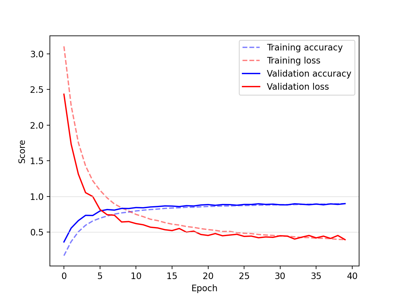
Across multiple runs the model has a loss (error) of about 0.4 and an accuracy of 0.9.

Parameters and network size

This network has about 36000 parameters. I find this interesting to think about, in particular when compared to the size of large language models (LLM) which are in the magnitudes of million (BERT, 2018), billions (GPT-3, 2020), or even trillion (PanGu-Σ, 2023) of parameters.

Deployment

The model is deployed as a REST API using Flask. The API accepts a POST request with a JSON payload containing the audio file encoded in base64. The audio file is decoded and saved to disk. The model is then loaded and used to predict the word. The prediction is returned as a JSON response.

The API is deployed on a Google Cloud Platform (GCP) VM instance configured with a static IP address. Since the API is accessed from a web browser, the API is exposed over HTTPS with a certificate issued by Let’s Encrypt, a free, automated, and open certificate authority (CA), run for the public’s benefit.

All the scripts and configuration files needed to deploy the API are available in the GitHub repository.

Conclusion

This project has served me to acquire some confidence in processing audio data with (deep) neural networks, as well as learning about the supporting infrastructure that supports the deployment of machine learning models. I’m grateful to Valerio Velardo for providing inspiration and learning resources. The source code can be found here.